Flowfield Art Based on Perlin Noise

Perlin noise is a pretty handy algorithm that can create many interesting generative arts, just like what I’ll introduce in this post. So, let me first introduce what is perlin noise.

What is Perlin Noise

Perlin noise is a type of gradient noise developed by Ken Perlin. It can produce random values with successiveness that resembles natural noise.

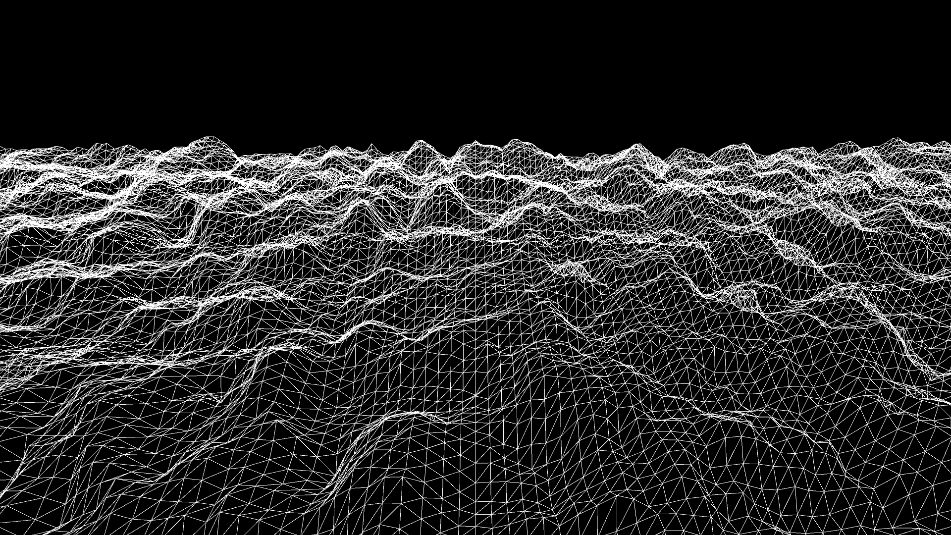
One example is to use perlin noise to generate terrain. Here is the 3D terrain created using perlin noise, and also Minecraft use such technique to generate terrain with randomness. Moreover, that’s why you can input specific seed to get same terrain - same coefficient will always create the same graph.

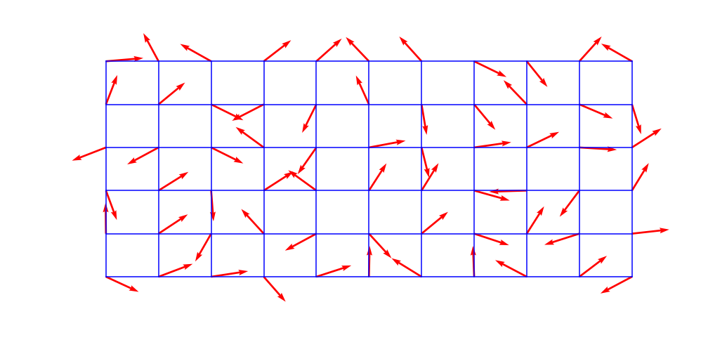
The algorithm can be separated into three steps, and I will use the 2D illustration on WikiPedia to explain:

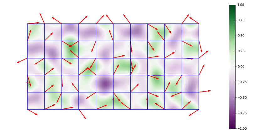
1. Define an n-dimensional grid where each grid intersection has associated with it a fixed random n-dimensional unit-length gradient vector, except in the one dimensional case where the gradients are random scalars between -1 and 1.

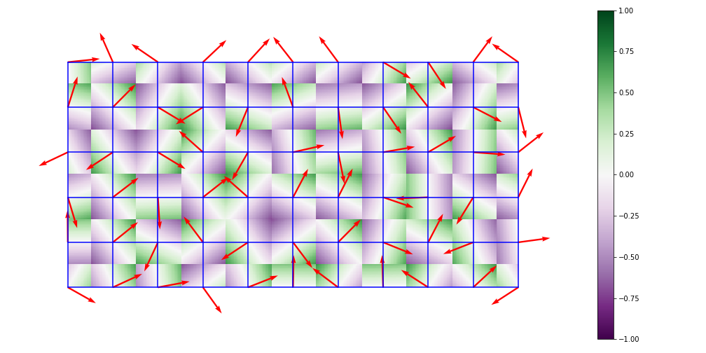
2. Take the dot product between its gradient vector and the offset vector to the candidate point. This dot product will be zero if the candidate point is exactly at the grid corner.

   For a point in a two-dimensional grid, this will require the computation of 4 offset vectors and dot products, while in three dimensions it will require 8 offset vectors and 8 dot products. In general, the algorithm has \(O(2^{n})\) complexity, where \(n\) is the number of dimensions.

3. Interpolate between $2^n$ points with function that has zero first derivative at the \(2^n\) grid nodes. It’s okay to just use linear interpolation, or smoothstep function for more natural performance.

Applying FLowfield and Particle System

Here is the tutorial video, where most following details are included

With perlin noise, we can get random 2D vector for each pixel value. Then, we can consider these vectors as force that particles would receive at those points, and this is exactly the idea of flowfield.

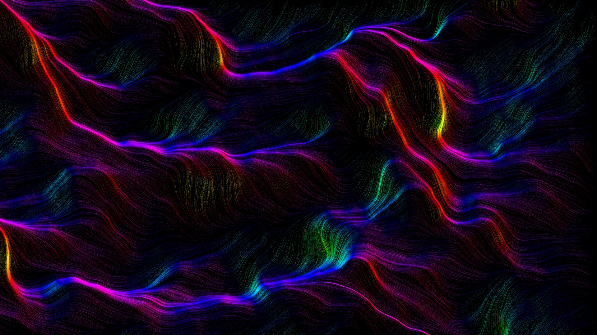
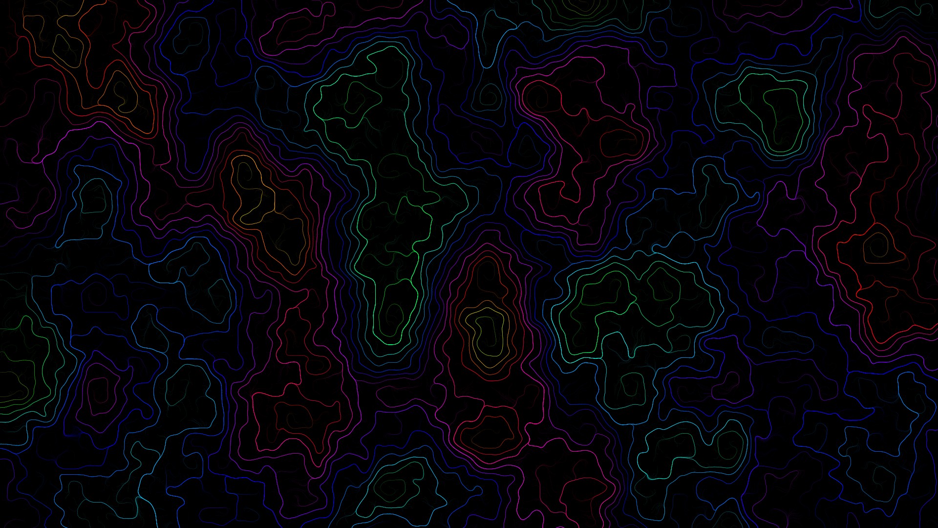
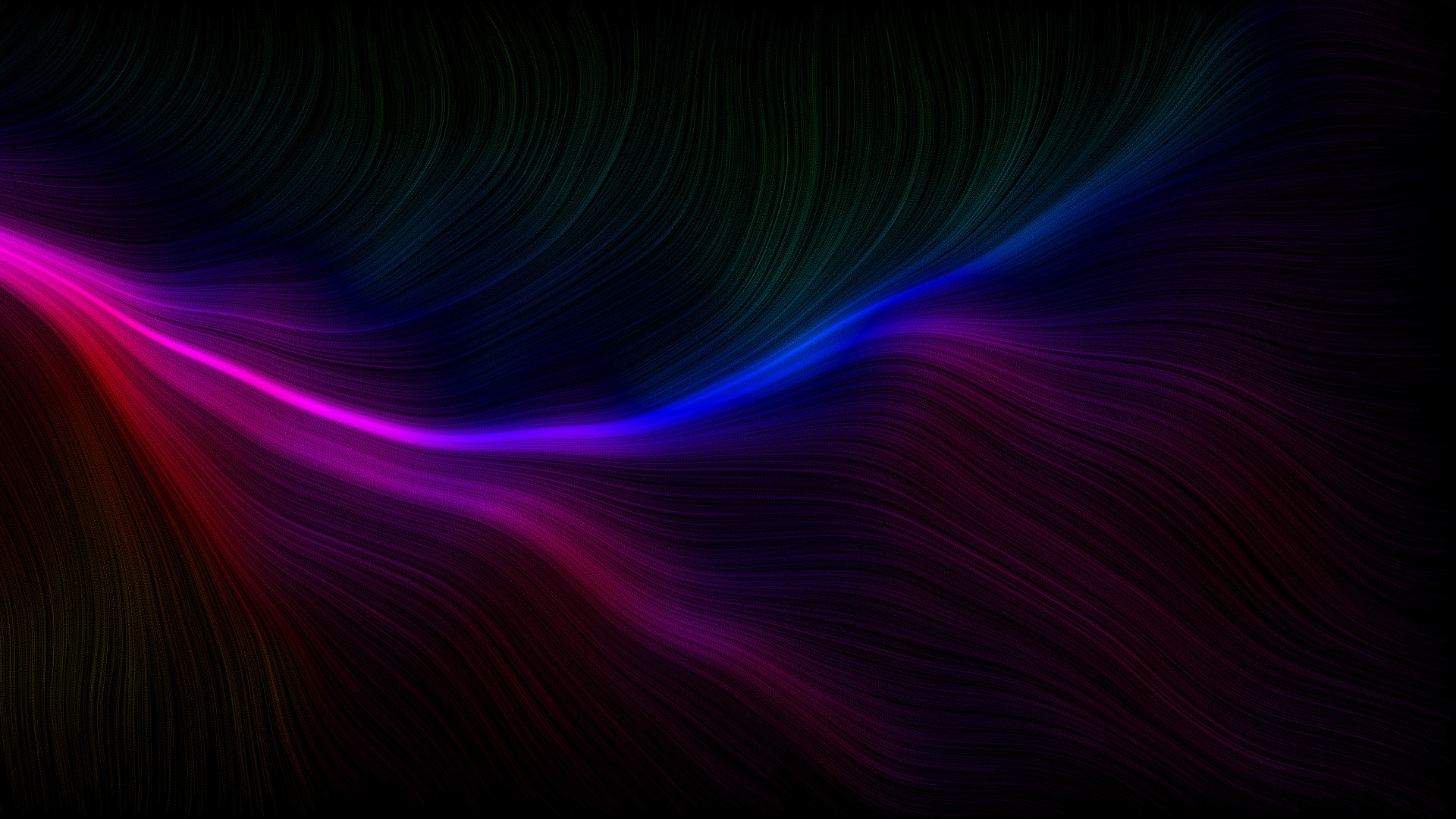
Here is the an arbitary flowfield I created:

You can think of those vectors as seaweed that drifts alongwith invisible water flows, where we can then add particles in.

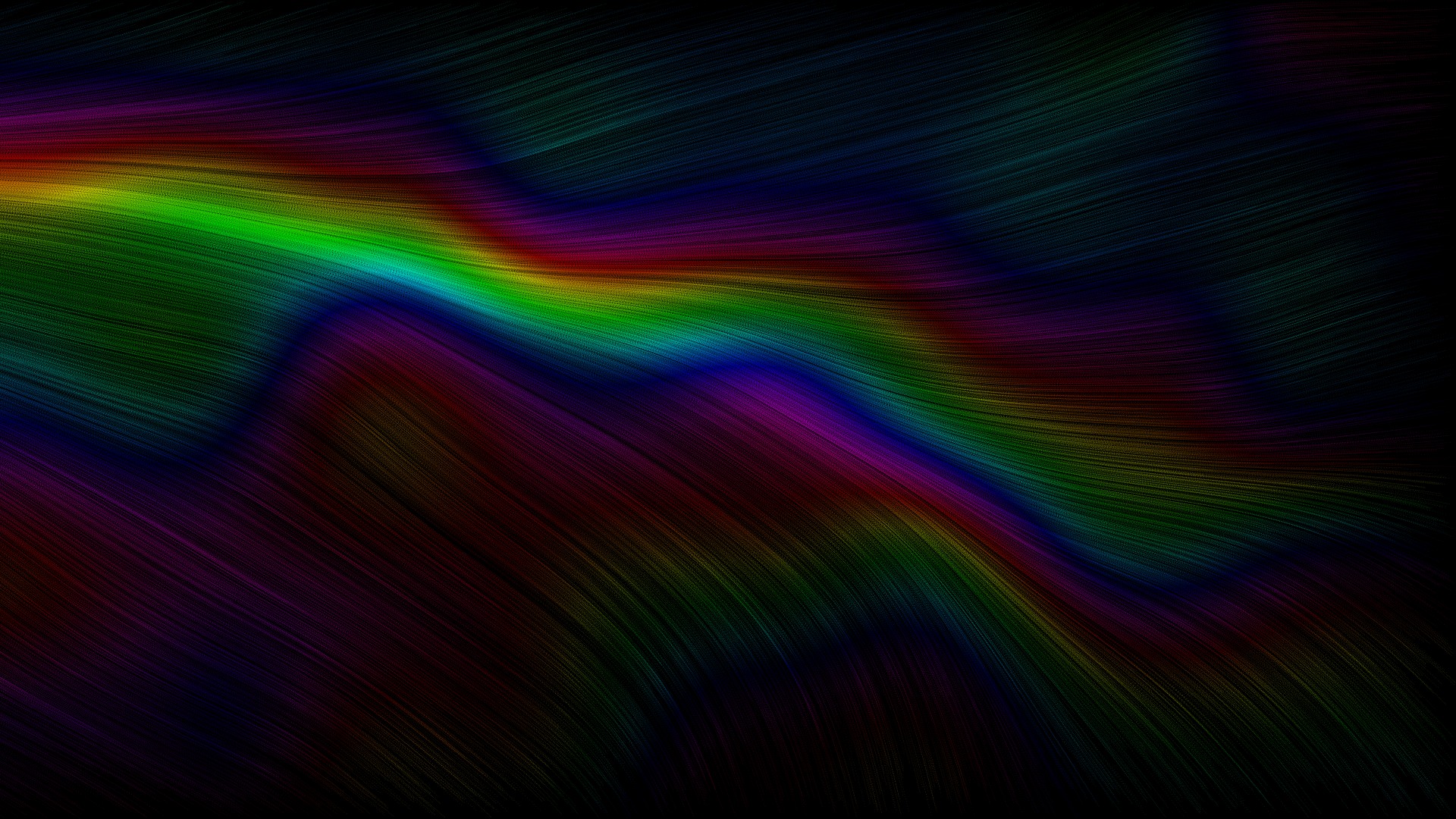
Finally, we can add particles in and draw their traces.

By applying HSB color settings according to their x postions, and adjusting all aspects of parameters like colorRange, interval length, particle size, particle amount… I can create interesting graphs with no limit!

Increasing Flowfield Variation

Increasing Color Range

Decreasing the Flowfield Force

Here is the complete code:

float angle = 0;
float strength = 0.005;
float noiseValue;
float speed = 100;
float angleMag = 1;
float colorFreq = 1.5;
float transparency = 150;

ArrayList<Particle> particles;

void setup() {
  fullScreen();
  background(0);
  colorMode(HSB);
  particles = new ArrayList<Particle>();
}

void draw() {
  for (Particle p : particles) p.update();

  if (particles.size() < 10000) {
    for (int i = 0; i < 10; i++)
      particles.add(new Particle(random(width), random(height)));
  }
}

class Particle {

  PVector pos;
  PVector vel;

  Particle(float x, float y) {
    pos = new PVector(x, y);
    vel = new PVector(0, 0);
  }

  void update() {
    if (pos.x < 0 || pos.x > width || pos.y < 0 || pos.y > height) 
      return;

    noiseValue = noise(pos.x * strength, pos.y * strength);
    vel = PVector.fromAngle(noiseValue * angleMag * TWO_PI);
    vel.setMag(speed);
    pos.add(PVector.div(vel, frameRate));
    display();
  }

  void display() {
    fill((255 * noiseValue * colorFreq) % 255, 255, 255, transparency);
    noStroke();
    ellipse(pos.x, pos.y, 0.5, 0.5);
  }
}